This project is carried out by me independently. The dataset is obtained publicly from Kaggle. All codes and their explanations are stored in my GitHub repository.
Project description
- Language: Python
- Libraries: sklearn, pandas, numpy, matplotlib, seaborn
- IDE: Jupyter notebook
- Project type: Machine learning, Unsupervised learning, K-Means clustering
FIFA 23 is a football video game created by Electronic Arts (EA). It became the best-selling football video game in Christmas UK retail charts. According to EA statistics, the game contains more than 700 teams with over 19,000 football players, playing in at least 30 football leagues. The data used in this project is taken from Kaggle. The objective of this project is to classify the players into various segments.
 Photo by Hatem Boukhit on Unsplash
Although I implemented this project just out of my interest in football and my general engagement in playing the FIFA video game, the results may be helpful for any external observer such that the valuation of players might be determined or justified based on the segment they are in. Additionally, a team’s success may be tested over the number of players from each segment with the purpose of finding out any correlation.
Data collection and cleaning
The dataset used initially contained 17,660 rows and 29 columns. In other words, 17,600 players were present in the dataset explained with 29 features. The features were both quantitative and qualitative, ranging from the player’s name to their market value. I first used Pandas to call the raw format of the CSV file from the GitHub repo. After careful observation of the dataset, I noticed that some players, who already retired from a club, are still shown as the players of that particular club. I decided to eliminate those players in order to have the most up-to-date statistics. To tackle this problem, an interesting point in the dataset helped me.
The already-retired players’ names start with their latest kit number (“15 Xavi”, “22 D. Alves”). This enabled me to separate those players by applying an algorithm to detect the player names that start with digits. The codes are as follows:
# This list object will store the indices of players whose names start with digit
player_indices_to_remove = []

# This loop iterates through the indices of all players to detect the ones with digit-starting player names
for index in fifa23_df.index.to_list():

    player = fifa23_df['Name'].loc[index]

    player_first_name = fifa23_df['Name'].loc[index][0]

    # If the player name starts with digit, it adds the index of that observation to removable indices list
    if player_first_name.isnumeric():

        player_indices_to_remove.append(index)

# Now, we drop the indices of players who are unnecesarily included in the dataset
fifa23_df.drop(player_indices_to_remove,axis=0,inplace=True)

# We reset the indices of the dataframe
fifa23_df.reset_index(drop=True,inplace=True)
The codes go over each player’s name by iterating through the indices of the observations, taking out the very first character of that name, and checking if that character is numeric. Later, indices of the positive cases are added to the previously created list that aims to store retired players. Subsequently, those players are dropped out of the dataset, and the indexing is re-set.
After tackling this problem, I faced yet another data problem. The numeric values indicating monetary values are put in with their respective currency and the prefixes, M and K, for millions and thousands, respectively. I needed to first eliminate the currency symbol and convert the values into their actual value. I formulated the below function that handles this specific duty:
def curreny_correction(column,dataframe, curreny_sign = str):

    # Split the value by the given currency symbol: euro in our instance

    splits = dataframe[column].str.split(curreny_sign, expand = True)[1]

    values = splits.str[:-1] # Store the values
    prefixes= splits.str[-1:] # Store the prefixes

    # Create a list object that will store the float-converted format of the values
    values_float = []

    for value, prefix in zip(values, prefixes):

        # The wage and value point are either in thousands (K) or millions (M) or 0

        if prefix == 'M': # Checks if letter is 'M' or the value is million

            try: # When values are zero, they cannot be converted into float and raises ValueError.
                 #I debug the coding for those occasions
                float_value = float(value) * 1000000
                values_float.append(float_value)

            except ValueError: # Adds just 0 when ValueError is raised
                float_value = 0
                values_float.append(float_value)


        elif prefix == 'K': # If the letter is 'K' or the value is thousands

            try: # When values are zero, they cannot be converted into float and raises ValueError.
                 #I debug the coding for those occasions
                float_value = float(value) * 1000
                values_float.append(float_value)

            except ValueError: # Adds just 0 when ValueError is raised
                float_value = 0
                values_float.append(float_value)

    # Returns the float values that are stripped of currency symbol and exponential letters
    return values_float
Features including “Value”, “Wage”, and “Release Clause” were converted using the above function. Different scripts were written to convert the features (“Position”, “Height”, “Weight”) with slightly different characters.
# Correcting 'Position' feature
fifa23_df['Position'] = fifa23_df['Position'].str.split('>', expand=True)[1]

# Correcting 'Height' feature
heigh_values = [float(value) for value in fifa23_df['Height'].str.split("cm", expand = True)[0]]
fifa23_df['Height'] = heigh_values

# Correcting 'Weight' feature
weight_values = [float(value) for value in fifa23_df['Weight'].str.split("kg", expand = True)[0]]
fifa23_df['Weight'] = weight_values
I eliminated 11 features based on whether they are non-useful for the analysis or have huge null values. The final dataset ready for the analysis contained 17 features and 10,104 observations.
Data visualization
I created a couple of pre-analytics graphs to get a better understanding of the data I am working with. Seaborn and matplotlib modules were used for visualization purposes.
Figure 1: Overall Rating Score of players per their Preferred Foot
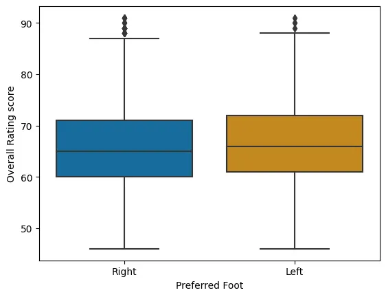
Figure 1 displays how the players are distributed on their rating score based on their preferred foot. There seems to be not a big difference between the feet. However, a very slight superiority can be observed for the left foot (presumably, because of Leo Messi the GOAT).
Figure 2: Scatter plot of Overall Rating Score and Age
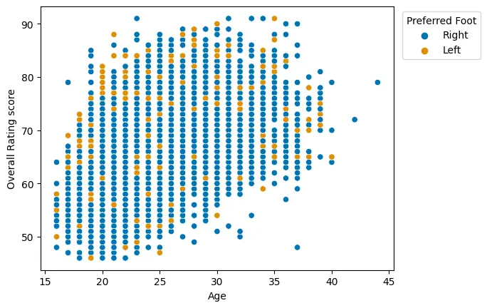
When it comes to the relationship between age and overall rating, an apparent positive linear relationship is visible (Figure 2). Seemingly, the greater the age of the player, the higher the rating is. The relationship seems to fade away after the age of 35.
Figure 3: Correlation matrix
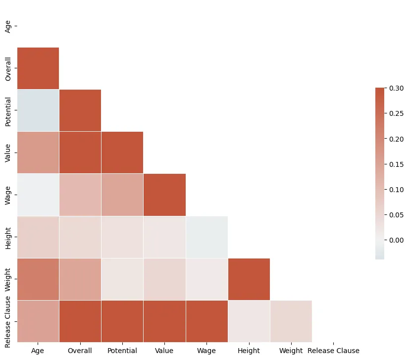
The correlation among the numeric variables of the dataset can be seen in Figure 3. High correlation scores are visible between Wage and Value, Height and Weight, Value and Overall, and Value and Potential. Although Overall Rating and Age are highly positively correlated, interestingly, there is not much correlation between Potential and Age. This signals that the young players who do not have high overall at the moment can increase their rating score substantially.
k-Means clustering
Initially, the numeric features need to be scaled, given the fact that the presence of outliers along with huge variations among the ranges of different variables can negatively impact the k-Means clustering process. I used StandardScaler from sklearn.preprocessing to standardize the quantitative variables.
For specifying the best number of clusters, I carried out Within-Cluster Sum of Squares (WCSS) and Average Silhouette methods.
Figure 4: WSCC method
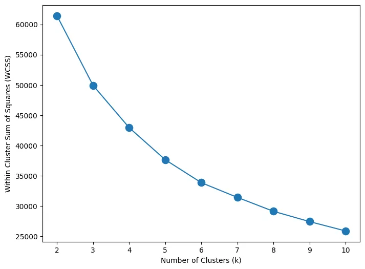
WSCC method calculates the cluster differences for each cluster number. By observing the above plot (Figure 4) for each k, it can be observed that the variations tend to slow down after around 5. Thus, the graph signals 5 to be the best number of clusters.
Figure 5: Average Silhouette method
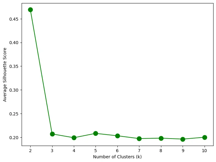
In the average silhouette method, the distances between neighboring cluster items and local cluster items are calculated. Figure 5 shows the final average silhouette scores for each k cluster number. Accordingly, the highest score signals the best k (besides 2).
As a result, I have enough proof to use 5 as my cluster number.
Project results: Final clusters
I used the kMeans function from sklearn.cluster to do the clustering. 5 different clusters were formed for the players in the dataset. The clusters and the number of players in each cluster are the following:
- Cluster 0 has 2640 players
- Cluster 1 has 3228 players
- Cluster 2 has 903 players
- Cluster 3 has 3197 players
- Cluster 4 has 136 players
Table 1: Cluster results
| cluster | Age | Overall | Potential | Value | Wage | Height | Weight | Release Clause |
|---|---|---|---|---|---|---|---|---|
| 0 | 20.47 | 56.40 | 67.42 | 386295.45 | 44692.80 | 180.29 | 72.88 | 7.700856e+05 |
| 1 | 23.80 | 67.22 | 73.81 | 2275497.21 | 14163.88 | 175.94 | 69.68 | 4.378210e+06 |
| 2 | 26.35 | 78.79 | 81.78 | 19393023.26 | 49131.78 | 182.18 | 75.93 | 3.738128e+07 |
| 3 | 25.44 | 66.95 | 72.08 | 1892169.22 | 15918.36 | 187.44 | 81.06 | 3.557997e+06 |
| 4 | 26.29 | 85.38 | 88.04 | 67459558.82 | 147213.24 | 182.27 | 76.98 | 1.309640e+08 |
Table 1 demonstrates how the players are separated based on the clusters.
Cluster 0 is characterized by younger players, who have relatively low rating scores and potential. Their values and wages are low, correspondingly. They are the kind of football players, who play in and are transferred by middle-sized clubs. Yet, they usually have a high release clause because of their young age.
Cluster 1 accommodates young and middle-aged players with yet low rating scores. These players usually start and end their careers in small- and middle-sized teams. However, given their still young age, they have a high release clause, as well.
Custer 2 has, on average, the oldest players among the clusters. The values and wages the players of this category have are fairly large, which signals their importance in the team. They mostly play in middle-sized and big teams, given their high values. Given their height and rating, I reckon that these are the strikes that play a crucial role in the attack.
Cluster 3 seems to have the same type of players as cluster 2. The difference is that cluster 3 players play in small- and middle-sized teams, explained by their low value and wage as well as low rating score and potential. They are quite tall and key players on the attack.
Cluster 4 takes the best players in the arena. They are still performing high and are the key players in their big teams. Arguably, they have been succeeding on their teams for quite a long time. Now, as they are old, their release clauses are also very low. Messi, Ronaldo, and Lewandowski should be in this cluster.