The objective of this project is to conduct a comprehensive analysis of Scottish schools in order to derive valuable insights. The analysis includes clustering and descriptive analysis, taking into account factors such as deprivation rate and total number of pupils. Additionally, an interactive map of Scotland has been developed to visually represent the location of each school. The clustering model has categorized local authorities into three distinct clusters based on average pupil count and deprivation score. The map highlights areas predominantly occupied by schools facing high levels of deprivation. The aim is to assist charities or non-governmental organizations (NGOs) involved in projects supporting these school pupils. All data used in this analysis is publicly available and sourced from the Scottish Government website. The Postcodes.io API was utilized to gather latitude and longitude coordinates for each school based on their respective postcodes. The codes for clustering, visualizations, map generation, and API application can be found in my GitHub repository. You are welcome to access and utilize the repository’s contents for personal or commercial purposes without seeking my consent. I hope you find this information enlightening and enjoyable to read.
Project description
- Language: Python
- Libraries: sklearn, pandas, numpy, matplotlib, seaborn, os
- IDE: Microsoft Visual Studio Code, Jupyter Notebook
- Project type: Machine learning, unsupervised learning, k-means clustering, data analytics, data visualisation
 Photo by Adam Wilson on Unsplash
The educational institutions in Scotland hold significant influence over the country’s economy. Scotland’s socio-demographic governmental structure places substantial emphasis on investing in the education of its population, as evidenced by the provision of free meals in all state schools. The economic status of local areas is largely determined by the location and prestige of state schools, with real estate prices being particularly dependent on this factor. Therefore, the level of deprivation in schools is a crucial determinant of areas that require further attention from either the government or non-governmental organizations. In this project, my objective is to assist concerned institutions in gaining a better understanding of the distribution of schools and the local authorities to which they are assigned.
I have undertaken two projects for Scottish schools, one of which involves the implementation of K-Means Clustering. The other project involves the creation of a map of Scotland that displays the schools, which can be accessed via this link or my Medium page (soon).
Schools Datasets Description
All data pertaining to the schools for this project has been sourced from the official statistics website of the Scottish Government. The consolidation of information regarding Scottish schools is based on three datasets:
- Postcode_deprivation: This dataset encompasses postcodes in Scotland along with their corresponding deprivation scores. Both pieces of information are utilized in this project. The dataset can be officially accessed from the following link.
- Scottish_schools_contact: This dataset comprises contact information for Scottish schools, including their respective postcodes. The project utilizes the postcode and seedcode associated with each school. The dataset can be officially accessed from the following link.
- Scottish_schools_stats: This dataset contains demographic statistics for Scottish schools. It has been formulated by merging various datasets. The data can be officially accessed from the following link.
Analysis
Descriptive analysis
Initially, a descriptive analysis was conducted on the collected information from schools. Subsequently, the datasets were merged and null values were dropped, resulting in a conclusion of 2,431 schools (out of 2,458 state schools in Scotland) with a total of 692,729 pupils. The average number of pupils per school was found to be 284.9, with a standard deviation of 309.7. The school with the highest number of pupils had 2,226, while the lowest school had no pupils at present. In terms of deprivation quintile, the average score was 2.8, with a standard deviation of 1.2. The number of schools falling under each deprivation quintile score is provided below:
- 1 quintile — 448 school
- 2 quintile — 507 school
- 3 quintile — 634 school
- 4 quintile — 557 school
- 5 quintile — 285 school
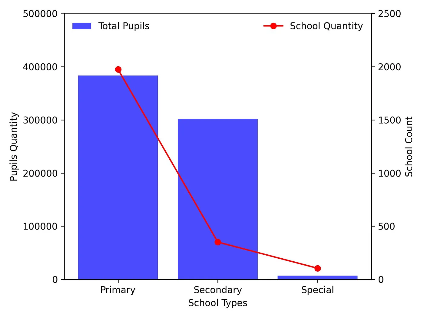
Figure 1: Total number of pupils and schools per school type
The data presented in Figure 1 illustrates the distribution of schools and pupils across various school types. It is evident that primary schools hold the majority in terms of both school count and pupil enrollment. Notably, the number of secondary schools is disproportionately low in comparison to the significant number of pupils. Special schools represent a minority within the overall distribution.
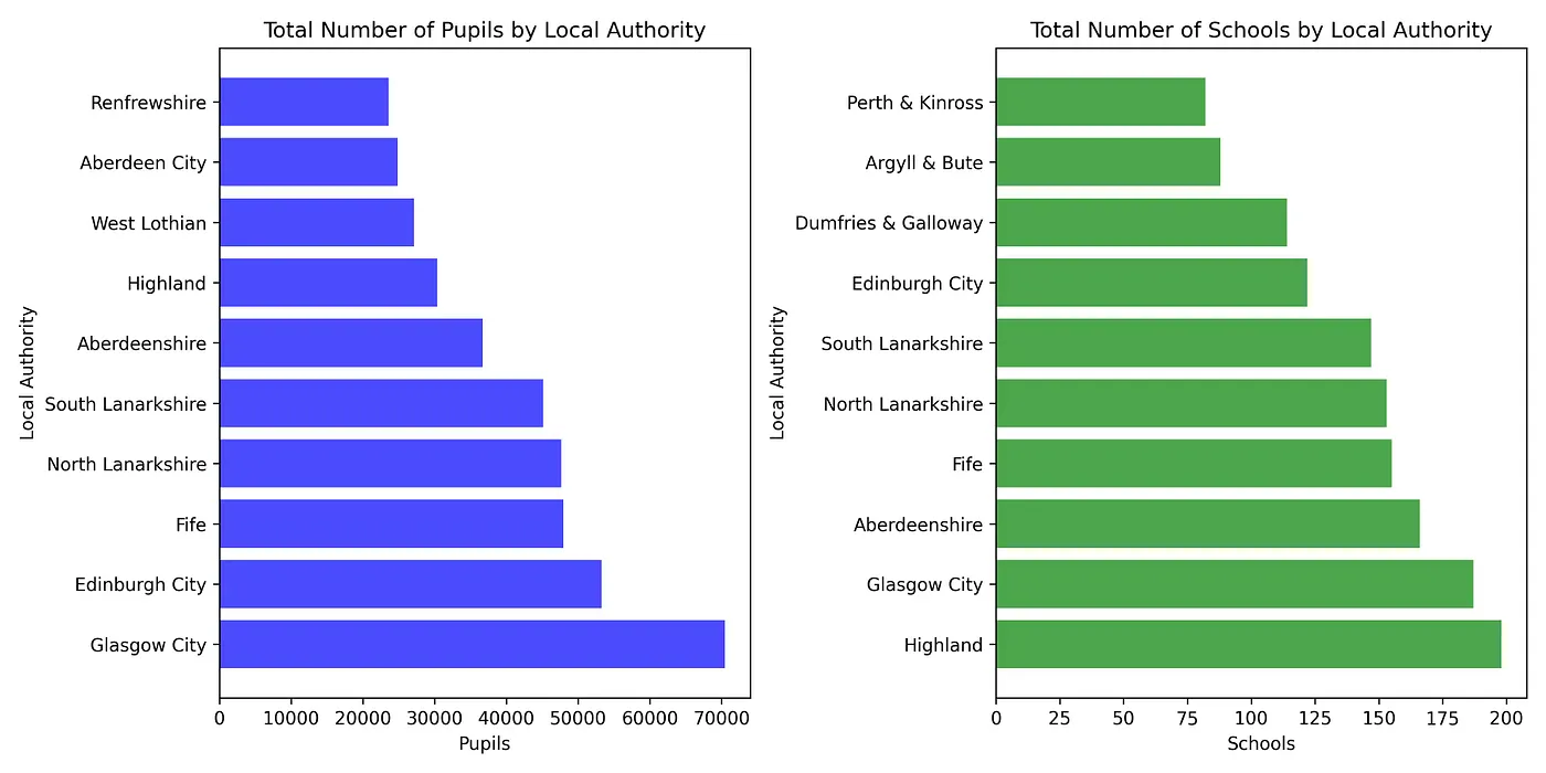
Figure 2: TOP10 Scottish local authorities with the highest number of pupils and schools
Figure 2 displays the pupil and school statistics for the top 10 local authorities. Notably, Glasgow city, Edinburgh city, and Fife emerge as the frontrunners in terms of pupil population, whereas Highland, Glasgow, and Aberdeenshire dominate the representation of schools. A noteworthy observation is the significant concentration of pupils in Edinburgh, the capital city of Scotland, despite the relatively lower number of schools. Conversely, Highland boasts the highest number of schools, despite having a comparatively smaller pupil population.
Unsupervised Learning: Clustering
Following the descriptive analytics, a discernible pattern emerged, enabling the categorization of local authorities based on their average deprivation score and average pupil count. To accomplish this, I proceeded to develop a data clustering algorithm utilizing unsupervised machine learning models. After careful consideration, I selected the k-Means clustering method due to its extensive applicability and widespread usage. Prior to implementing the clustering technique, I performed an initial data transformation to ensure optimal results.
Preprocessing before Clustering
Due to the significant disparity in numerical values observed, with deprivation scores ranging from 1 to 5 and total pupil counts ranging from 0 to over 2000, I made the decision to normalize these values in order to enhance the efficiency of the clustering process. To accomplish this, I employed the StandardScaler object from the sklearn module.
# Import standard scaler to z-score normalize the data
from sklearn.preprocessing import StandardScaler

# specify the numerical features
numeric_columns = ['Pupils', 'DeprivationScore']

# Create a scaler object
scaler = StandardScaler()

# Scale the numeric columns
scaled_values = scaler.fit_transform(df[numeric_columns])

# Sonvert the numpy array of scaled values into a dataframe
scaled_values = pd.DataFrame(scaled_values, columns = numeric_columns)
Finding k: the optimal number of clusters
When considering k-Means clustering, a crucial step is determining the number of clusters (k), which must be predetermined. However, identifying the optimal k is not a straightforward process and requires both domain knowledge and technical expertise. Given the lack of personal expertise in the school industry, I chose to rely on my technical knowledge. To ensure the accuracy of k, I employed two different methods to determine the best value. To achieve this objective, I utilized the Within-Cluster Sum of Squares (WCSS) and Average Silhouette Method.
Within-Cluster Sum of Squares method
The WCSS method assesses the variations within each cluster by summing the squared differences between values. By testing different k values, it compares the differences in WCSS scores and selects the value at which the subsequent scores stabilize. The code implementation for this method is as follows:
# Create a list to store WCSS values
wcss = []

# Iterate in a range from 2 to 10, inclusive
for k in range(2, 11):
    km = KMeans(n_clusters = k, n_init = 25, random_state = 1234) # Create a cluster object for each k
    km.fit(scaled_values) # Fit the scaled data
    wcss.append(km.inertia_) # Add the inertia score to wcss list

# Convert the wcss list into a pandas series object
wcss_series = pd.Series(wcss, index = range(2, 11))

# Draw a line chart showing the inertia score, or WCSS, for each k iterated
plt.figure(figsize=(8, 6))
ax = sns.lineplot(y = wcss_series, x = wcss_series.index)
ax = sns.scatterplot(y = wcss_series, x = wcss_series.index, s = 150)
ax = ax.set(xlabel = 'Number of Clusters (k)',
            ylabel = 'Within Cluster Sum of Squares (WCSS)')
The provided codes generate Figure 3, which allows for the observation that the scores exhibit minimal variation beyond the value of 3. Consequently, it can be inferred that 3 is the optimal k, as determined through the utilization of the WCSS method.
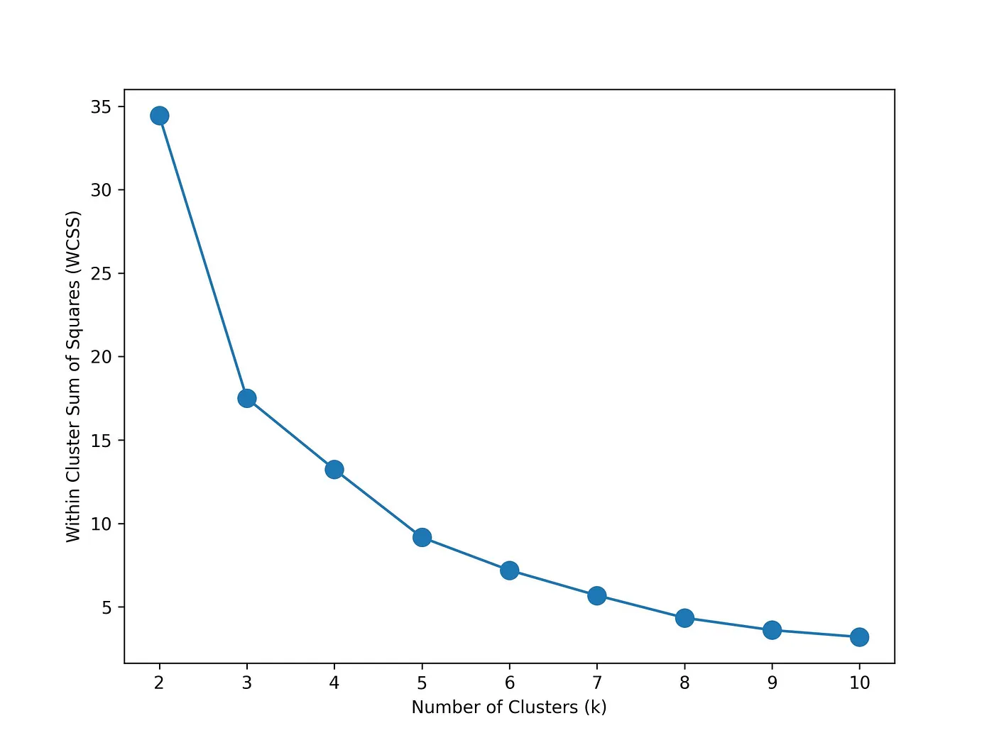
Figure 3: Within-Cluster Sum of Squares method results
However, this cannot be the sole basis for formulating three clusters. Therefore, it is necessary to run the Silhouette method as well.
Silhouette method
The Silhouette method measures the similarity of a data point within its own cluster in comparison to other clusters. For each data point, it calculates its distance from its local points (a) and neighboring points (b). It then applies the formula (b-a)/max(a,b) to calculate the Silhouette score. The average Silhouette scores of all the points within one cluster determine the final score. A higher Silhouette value indicates better locality and thus a better cluster count. The code implementation for this method is as follows:
# Import silhouette_score function
from sklearn.metrics import silhouette_score

# Create a list to store silhouette values
silhouette = []

# Iterate in a range from 2 to 10, inclusive
for k in range(2, 11):
    km = KMeans(n_clusters = k, n_init = 25, random_state = 1234) # Create a cluster object for each k
    km.fit(scaled_values) # Fit the scaled data
    silhouette.append(silhouette_score(scaled_values, km.labels_)) # Add the silhouette score to silhouette list

# Convert the silhouette list into a pandas series object
silhouette_series = pd.Series(silhouette, index = range(2, 11))

# Draw a line chart showing the average silhouette score for each k iterated
plt.figure(figsize=(8, 6))
ax = sns.lineplot(y = silhouette_series, x = silhouette_series.index, color='green')
ax = sns.scatterplot(y = silhouette_series, x = silhouette_series.index, s = 150, color='green')
ax = ax.set(xlabel = 'Number of Clusters (k)',
            ylabel = 'Average Silhouette Score')
Figure 4 below represents the outcome of the aforementioned codes, displaying the results of Silhouette testing. The chart unequivocally indicates that 3 possesses the highest average silhouette score. Consequently, this test execution ultimately determines 3 as the optimal value for k, as well.
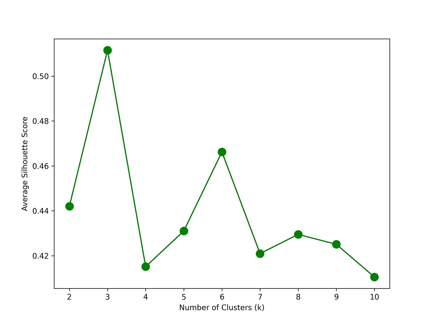
Figure 4: Silhouette method results
As both tests have indicated that the optimal value for k is 3, we can proceed with confidence to implement clustering with 3 clusters. The subsequent sub-section will construct the k-Means clustering and elucidate its outcomes.
k-Means clustering
In order to construct the model, the KMeans object from the sklearn library was utilized. The implementation of this object can be achieved through the following code:
# Create kmeans object
km = KMeans(n_clusters = 3, n_init = 25, random_state = 1234)

# Fit the scaled values
km.fit(scaled_values)
The parameter ’n_init’ determines the number of times the algorithm will be executed with different initializations of cluster centroids. Increasing this value is recommended in order to achieve better clustering results. After conducting multiple tests, it was determined that a value of 25 is sufficient for this project. The ‘random_state’ parameter is used to control the randomness or randomness seed for various operations involving randomness. It is advisable to set it to 1234 for most machine learning models. Among the three constructed clusters, Cluster 0 consists of 5 local authorities, Cluster 1 consists of 15 local authorities, and Cluster 2 consists of 13 local authorities.
Table 1: Clustering results
| cluster | Pupils | DeprivationScore |
|---|---|---|
| 0 | 438.29 | 3.50 |
| 1 | 331.48 | 2.39 |
| 2 | 175.87 | 3.31 |
The clustering results can be found in Table 1.
Cluster 0
This is the first cluster and is characterized by a relatively high number of pupils and a higher deprivation score. In other words, these are localities with a low level of deprivation but a large number of pupils. Despite the high number of pupils, these localities are relatively less deprived.
Cluster 1
This group of localities also has a large number of pupils, but the average deprivation score is the lowest among the three clusters. This indicates that the local authorities in this category require the most attention.
Cluster 2
The localities in this group have a lower number of pupils but a fair deprivation score. This group likely requires the least attention, as they are not highly deprived and the pupil count is not significant.
The scatter plot in Figure 5 illustrates the assignment of each locality to its respective cluster.
Zoom image will be displayed
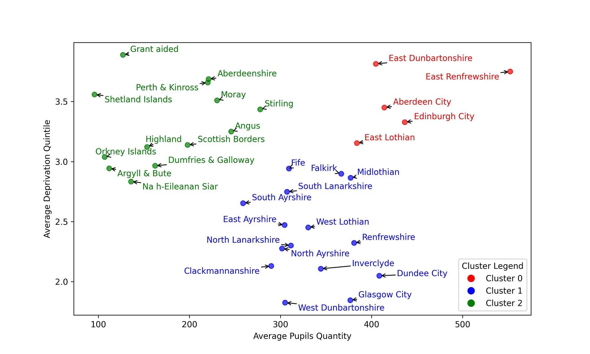
Figure 5: Scottish local authorities clustering
The complete list of localities in each cluster is provided below:
- Cluster 0: Aberdeen City, East Dunbartonshire, East Lothian, East Renfrewshire, Edinburgh City
- Cluster 1: Clackmannanshire, Dundee City, East Ayrshire, Falkirk, Fife, Glasgow City, Inverclyde, Midlothian, North Ayrshire, North Lanarkshire, Renfrewshire, South Ayrshire, South Lanarkshire, West Dunbartonshire, West Lothian
- Cluster 2: Aberdeenshire, Angus, Argyll & Bute, Dumfries & Galloway, Grant aided, Highland, Moray, Na h-Eileanan Siar, Orkney Islands, Perth & Kinross, Scottish Borders, Shetland Islands, Stirling
Conclusion
I had two primary objectives in undertaking this project:
- Personal development — My aim was to showcase my abilities and enhance my career prospects by implementing similar projects and gaining valuable experience.
- Educational exploration — As an international citizen of Scotland, I was keen to deepen my understanding of the country’s educational system. Additionally, I am actively involved in a charity organization that carries out projects for Scottish schools.
If you found this project insightful and beneficial, I encourage you to show your appreciation by clapping and sharing it with your peers. Furthermore, feel free to utilize the project for your personal and professional purposes without seeking my consent, as I am a strong advocate of open-source projects and actively contribute to the community.
Should you have any questions, concerns, or suggestions, please do not hesitate to comment below or contact me via email at ezeynalli@hotmail.com.